
William F. Campbella, Christopher M. Hartmana,b, Hui Christophersena
aU.S. Naval Research Laboratory, Marine Meteorology Division, Monterey, CA
bSAIC, Monterey, CA
The Earth observing system is rapidly changing from a few, long-lived, well-calibrated, but expensive legacy satellites towards many smaller, more flexible, and less expensive microsats. A constellation of microsats can provide a high volume of high temporal resolution data, fill data gaps, and mitigate risk via data redundancy, but large data volumes can also be problematic for a real-time NWP system. Most global NWP centers average (superob) observations, or discard (thin) a large percentage of them, or both. The reasons are not simply about data volume. Spatially correlated error is very difficult to account for properly, and ensuring that two profiles from the same satellite and instrument have a certain minimum horizontal spacing can mitigate the effect of that error. Another reason to thin is to choose good data, which is generally more about avoiding bad data. QC procedures can be expensive to run on full, raw radiance datasets, so often there is a thinning step first, which could potentially throw out all of the good data in a small area, leaving only bad data. We will present an adaptable methodology to address all of these concerns in a timely fashion, and show experiments comparing the performance of traditional data thinning versus the new approach. Note that this method is not restricted to satellite radiances, and is equally applicable to legacy instruments and newer microsats.
Specifically, we perform a static thinning in an observation-blind way, retaining, for a particular satellite and instrument, approximately five times more data than we do routinely in our operational NWP system (NAVGEM). These data are chosen to fall near the centers of an approximately equal area latlon grid. The next steps are the new graph-theoretic approach to retain as many observation locations as possible while respecting an observation density function both globally and locally. This is done by first choosing a normalized observation density function whose maximum is determined by the minimum safe horizontal distance needed to mitigate spatially correlated error, chosen by the user. Other aspects of the density function can be set by the user as well. For instance, one might want the maximum density of observations over the SH and tropical oceans, less dense observations over NH oceans, and even less dense observations over land. Once the density function is set, each observation location is assigned a radius inversely proportional to the square root of the density function. At that point other metadata, such as QC flags, can be considered, possibly inflating the assigned radius for suspect obs. Because large radius observations are less likely to be chosen (see algorithm description below), QC inflation of observation radii downweights their selection, unless they are the only available observation, which is the behavior that we desire.
Once the radii are assigned, we can solve the maximum disjoint set problem on the sphere. If one were to plot circles of the assigned radius at each observation location, there will be many circles that overlap, indicating that the observations are too close to one another relative to the assigned density function. The maximal disjoint set problem solution is to retain as many observations as possible with no circle overlapping any other circle. In general, this is an NP-hard problem, but fast, approximate methods work very well. We construct a graph representation of the observations, where each observation location is a node, and each overlapping circle is an edge between two nodes. Then we apply the algorithm to judiciously eliminate nodes until we are left with a completely disjoint set of nodes, (nearly) the maximum number of observations. These observations will directly reflect the chosen density function both locally and globally.
We plan to present results from cycling DA runs of NAVGEM for satellite radiances using our standard thinning at baseline resolution, graph thinning at that same (uniform) resolution, and graph thinning at the same average resolution, but distributed according to density functions of interest.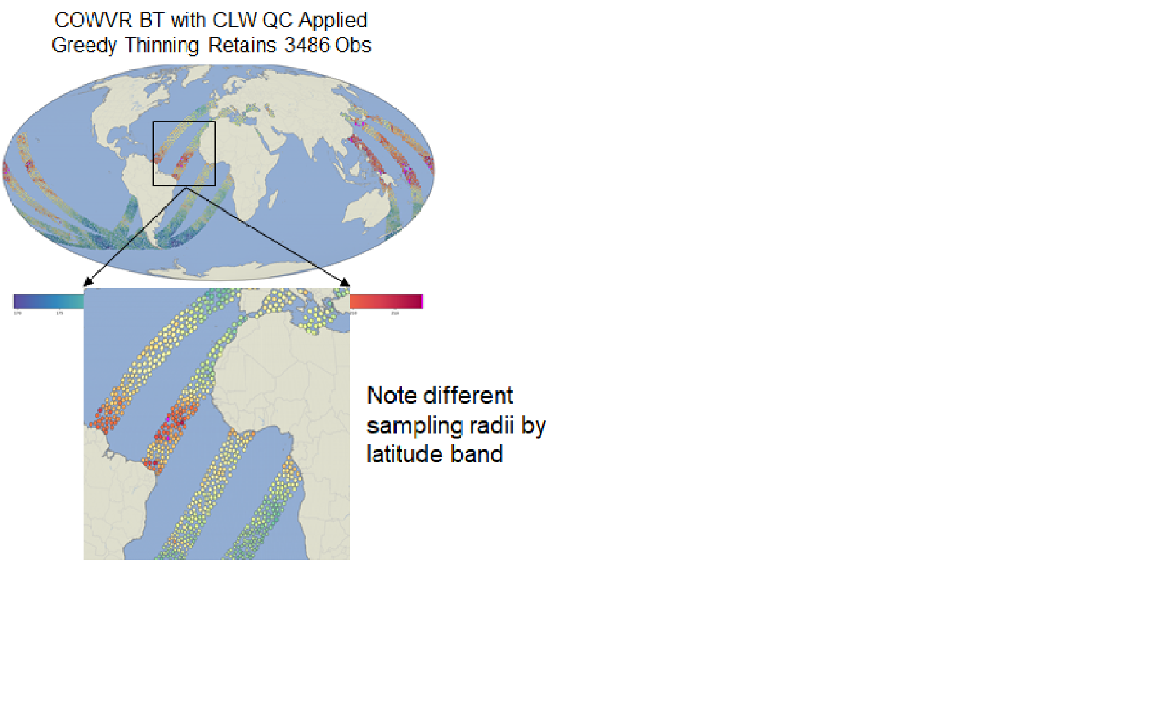
 - Indicates paper has been withdrawn from meeting
 - Indicates an Award Winner